To plot distributions

To plot distributions and to do physical cut, the user should understand a little bitter about the momentum setting. The momentum setting is as following:

  namel   :='(ef efb wb h0 w);                 
  momentum:=  p1 p2  p3 p4 p5

where all the momentum are in the laboratory frame. In the case of two initial particles, z-axial is the beam direction. In the case of one initial particle z-axial is of no special meaning.

The components of n-th momentum is:

      p(1,n),  the energy component
      p(2,n),  x-axial component
      p(3,n),  y-axial component
      p(4,n),  z-axial component

There are four quantity defined in FDC as following:

$cos\theta$:

  examples:
      wcos(p3,p4) means cos of the angle between p3 and p4
      wcos(p3,z)  means cos of the angle between p3 and z-axial
      wcos(p4,x)  means cos of the angle between p4 and x-axial 
      ......
      wcos_lorentz(p4,p3,p3+p5) means then cos of angle between p4,p3
                  in the center-mass frame of p3+p5.

s: is the invariant mass, which is defined as

$sqrts(pn)=\sqrt{p(1,n)^2+p(2,n)^2+p(3,n)^2+p(4,n)^2}$

  examples:
      sqrts(p3,p4) means the invariant mass of p3 and p4
      sqrts(p3,p4,p5) means the invariant mass of p3,p4 and p5 
      ......

pt: is the transverse momentum, which is defined as

$pt(pn)=\sqrt{p(2,n)^2+p(3,n)^2}$

  examples:
      pt(p3) means the transverse momentum of p3
      pt(p3,p4) means the transverse momentum of p3 and p4 
      ......

vpt: is the pseudo-velocity, which is defined as

$vpt(pn)={1 \over 2} log{p(1,n)+p(4,n) \over p(1,n)-p(4,n)}$

  examples:
      vpt(p3) means the pseudo velocity of p3
      vpt(p3,p4) means the pseudo velocity of p3 and p4 
      ......

There are two kind of ways to describe the distributions. One is to plot distributions visa the four well defined quantity described above. In this case, the boundary can be find out out by the FDC, therefore it will use the default boundary if the user do not give the boundary. The format of each line is

   {n,a,mg,name}
   {n,a,mg,b0,b1,name}

where the "n" means the n-th distribution, "a" is the $cos\theta$ or $s$, or $pt$ or $vpt$ variable visa which the distribution is plotted, "mg" means to divide the variable range into "mg" grids, and "name" is just the name given by the user to refer to the distribution. b0 and b1 are the upper and lower boundary respectively.

Another is to plot distributions visa ambitory expressions of momentums (include the four well defined quantities). In this case, the boundary of the variable must be inputed. The format of each line is

   {n,a,mg,b0,b1,name}

where the "n" means the n-th distribution, "a" is a kind of expression of variable visa which the distribution is plotted, "mg" means to divide the variable range into "mg" grids, "b0" is the lower boundary of "a", "b1" is upper boundary of "a", and "name" is just the name given by the user to refer to the distribution.

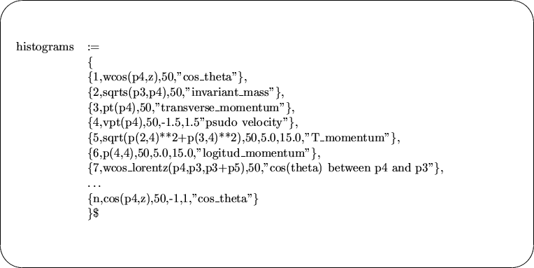
The following is an example. To obtain the distributions, the following part must be added to the input file "process.def".

where the line 1 is to ask for the distribution visa the cos of the angle between p4 and z-axial, "50" in the line means to divide the variable range into 50 grids, and "cos_theta" is just the name given by the user to refer to the distribution. The above line number 2 is to ask for the distribution visa the invariant mass of p3 and p4, and more similar lines could be added.

The following is an example. To obtain the two dimension distributions, the following part must be added to the input file "process.def".

Where the format of each line is

   {n,x,y,mx,my,name}
   {n,x,y,mx,my,x1,x2,y1,y2,name}

where the "n" means the n-th distribution, "x" and "y" are the $cos\theta$ or $s$, or $pt$ or $vpt$ variable visa which the distribution is plotted, "mx" and "my" means to divide the variable range into "mx" and "my" grids, and "name" is just the name given by the user to refer to the distribution. x1 and x2 are the upper and lower boundary of x respectively. y1 and y2 are the upper and lower boundary of y respectively.